Now that we’ve seen how a nonlinear 1D signal can be made linear by using Vandermonde interpolation, we can quickly expand our discussion to images by treating each pixel as a 1D function of intensity to be corrected.
Let’s first see how a nonlinearity introduced in our project data is reflected in the reconstructed image…
We start with a simplified model of beam hardening described in: https://aapm.onlinelibrary.wiley.com/doi/full/10.1118/1.2742501
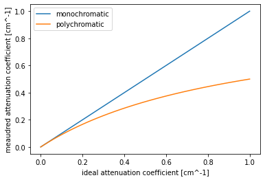
where the polychromatic attenuation coefficient \(\langle \mu \rangle\) can be modeled in terms of the true attenuation coefficient \(\mu\) and penetration distance \(x\)
Note: \(\lambda\) is a fitting parameter (not wavelength) that controls the strength of beam hardening. If \(\lambda = 0\) then there is no beam hardening. If $= $ then \(\langle \mu \rangle = 0\)
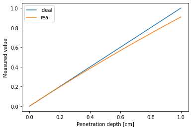
Limitation: Because we cannot easily separate \(x\) and \(\mu\) we know that in the ideal case \(-ln(I/I_0) = \int \mu dx\) thus here we need to make the assumption that materials have about equal \(\mu\) (i.e.) that \(\mu\) doesn’t contribute to beam hardening (which we know not to be true because bone will harden more than water). But we’ll make this assumption just for this demonstration.
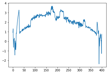
import numpy as npimport matplotlib.pyplot as plt%matplotlib inlinex = np.linspace(0, 1)lam =0.1#set small amount of beam hardeningmu = xdef beamHardening(x, lam=1): #here we cannot separate mu and penetration distance so we have to assume them to be equalreturn x/(1+lam*x)plt.plot(x, mu, label='ideal')plt.plot(x, beamHardening(x, lam), label ='real')plt.xlabel('Penetration depth [cm]')plt.ylabel('Measured value')plt.legend()plt.show()
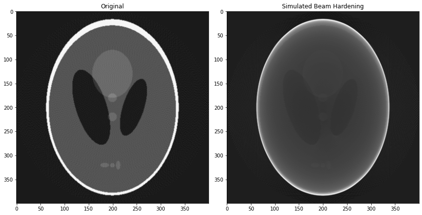
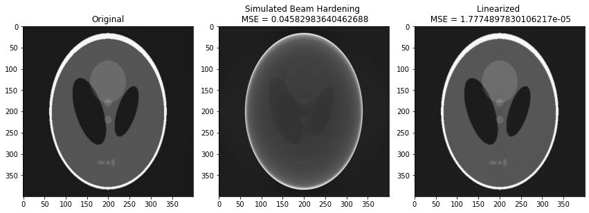
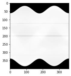
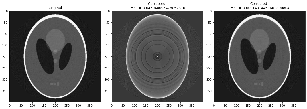
from skimage.data import shepp_logan_phantomfrom skimage.transform import radon, rescale, iradonp = shepp_logan_phantom()p = rescale(p, scale=1, mode='reflect', multichannel=False)theta = np.linspace(0., 360., 360, endpoint=False)r = radon(p, theta=theta)ideal = iradon(r, theta=theta)corrupted_r = beamHardening(r, lam=0.1) #here we cannot separate mu and penetration distance so we have to assume them to be equaluncorrected = iradon(corrupted_r, theta=theta)fig, (ax1, ax2) = plt.subplots(1, 2, figsize=(12, 6)) ax1.set_title("Original")ax1.imshow(ideal, cmap=plt.cm.Greys_r)ax2.set_title("Simulated Beam Hardening")ax2.imshow(uncorrected, cmap=plt.cm.Greys_r)fig.tight_layout()plt.show()
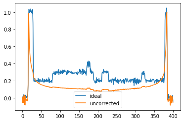
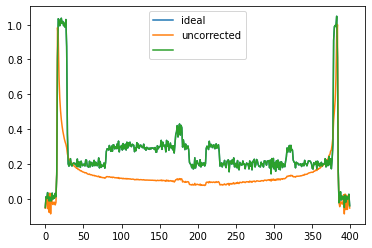
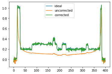
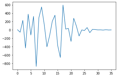
idealLine=ideal[:,int(ideal.shape[0]/2)]uncorrectedLine=uncorrected[:,int(ideal.shape[0]/2)]uncorrectedLine/=max(uncorrectedLine) #normalized for easier comparisonplt.plot(idealLine)plt.plot(uncorrectedLine)plt.legend(["ideal","uncorrected"])plt.show()
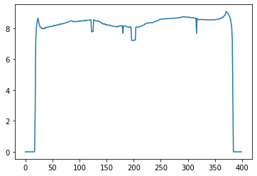
print(correctionLineFunc.shape)print(corrupted_r.shape)pc = np.zeros([corrupted_r.shape[0], corrupted_r.shape[1]])for i in np.arange(1,corrupted_r.shape[1]): pc[:,i] = corrupted_r[:,i]*correctionLineFunc
(400,)
(400, 360)
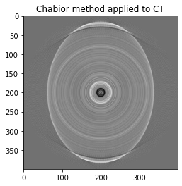
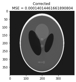
chabior_corrected = iradon(pc, theta=theta)plt.imshow(chabior_corrected, cmap ='gray')plt.title("Chabior method applied to CT")plt.show()
In our first imaging example we will start by fitting one polynomial fit function to applied to uniformly to every pixel in our 400x400 pixel image.
We can generate our new Vandermonde matrix, let’s start with \(n=3\) monomial terms, since each image has \(400^2=160000\) pixels our matrix will look like
def poly_recon(A, theta):"""Argument is projection vandermonde matrix [proj.ravel() X view angles] and theta array, returns recon.ravel() X deg matrix of vandermonde recons""" deg=A.shape[1] sz =int(A.shape[0]/theta.size) A=A.reshape([sz,theta.size,deg]) f = np.zeros([sz*sz,deg])for i inrange(deg): fi=iradon(A[:,:,i],theta=theta, circle=True) f[:,i]=fi.ravel()return fdef vanderRecon(proj, theta, deg):"""Argument is [xpix*ypix X theta] projection, returns [recon.ravel() X deg] matrix of vandermonde reconstructed projections""" A=np.vander(corrupted_r.ravel(),deg, increasing=True)return poly_recon(A,theta);
Let’s confirm that the size of the Vandermonde matrix of our recons is what we expect…
deg=3#set number of monomial termsA = vanderRecon(corrupted_r, theta, deg)print(A.shape)
(160000, 3)
A_rank = np.linalg.matrix_rank(A)print(A_rank)
3
Now let’s define our correction function once we determine our coefficients and a loss function to define our mean squared error MSE
deg =6f = vanderComborecon(corrupted_r,m,theta, deg)print("The Vandermonde matrix has a shape of [{0:d}, {1:d}] and a condition number of: {2:.0f}".format(f.shape[0], f.shape[1], np.linalg.cond(f)))
The Vandermonde matrix has a shape of [160000, 36] and a condition number of: 3367960979906
Note that the condition number of the \(qm\) matrix is very large, meaning that it is pretty poorly conditioned, thus our algorithm will be very sensitive to different input values. Is there a way to decrease the condition number and better condition our problem?
Condition number is a measure of the sensitivty of a problem to error in input. A large condition number number indicates an unstable result that could vary drastically depending on minor errors in the input.
A large condition number is a known problem of vandermonde matrix inversions.
Looking at our coefficients above and how large and widely varying they are is a result of the problem being poorly conditioned, not only do these coefficients vary widely with small changes in input (try re-running the program again with noise added), but also the coefficients aren’t very intuitive at all.
def square(c):return c.reshape([int(np.sqrt(len(c))), -1])def performCorrection2D(corrupted_r, m, c):return np.polynomial.polynomial.polyval2d(corrupted_r.ravel(), m.ravel(), square(c)).reshape(corrupted_r.shape)
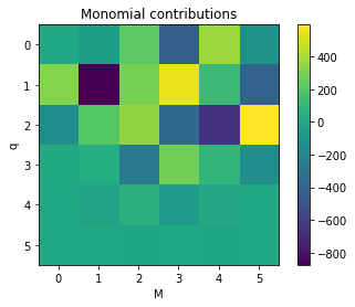
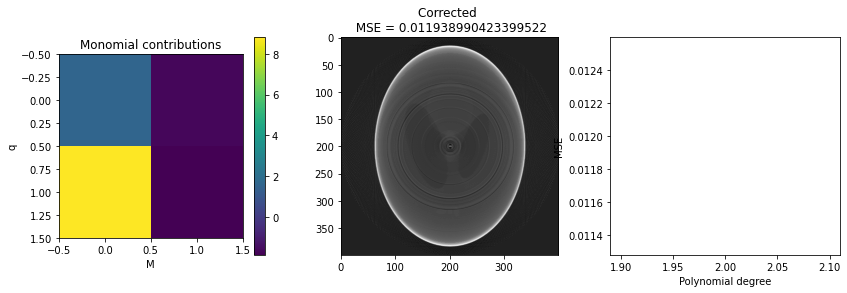
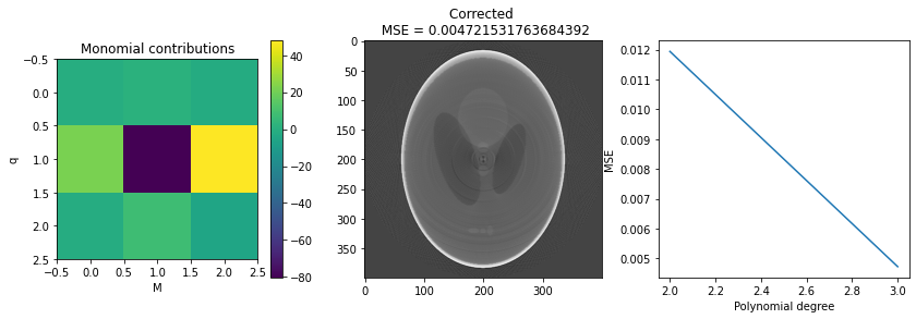
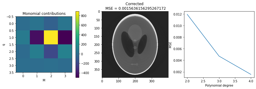
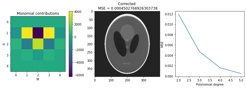
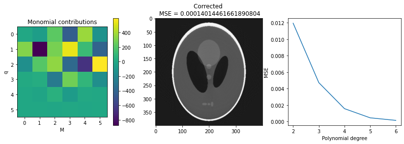
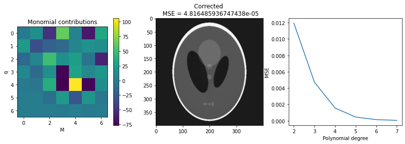
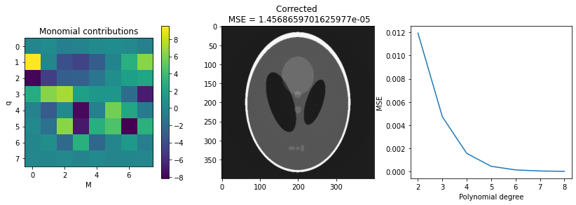
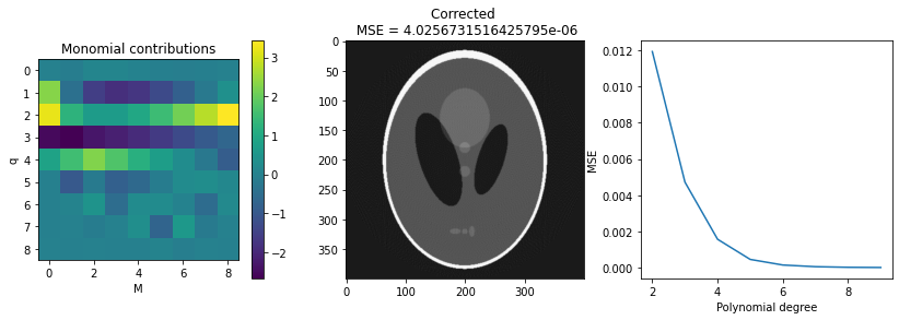
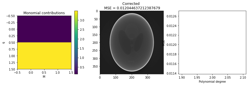
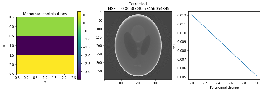
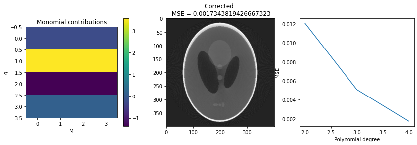
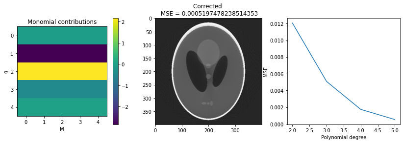
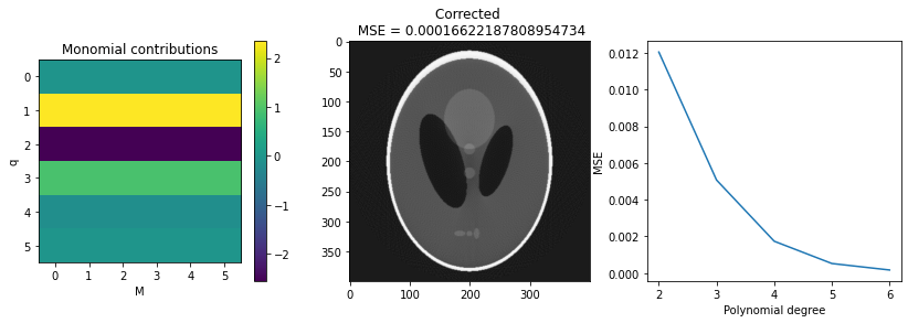
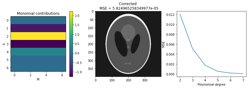
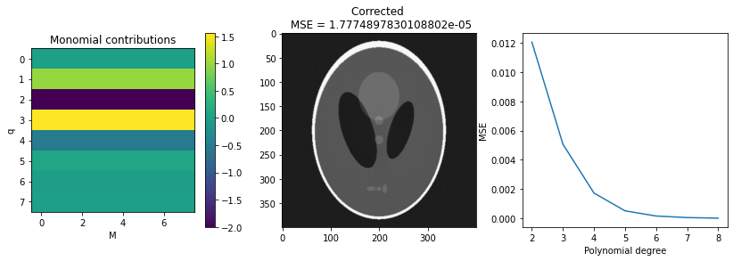
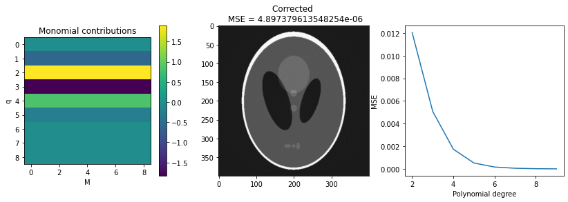
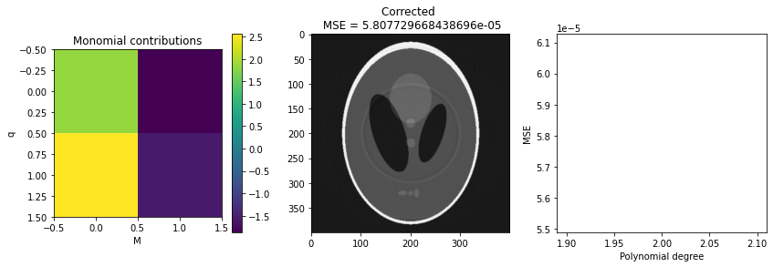
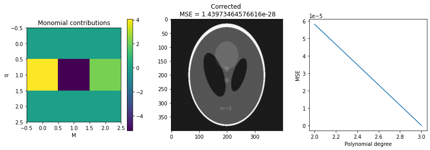
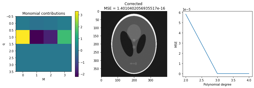
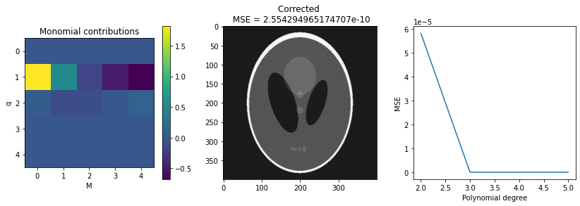
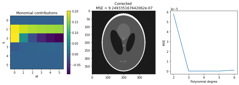
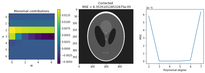
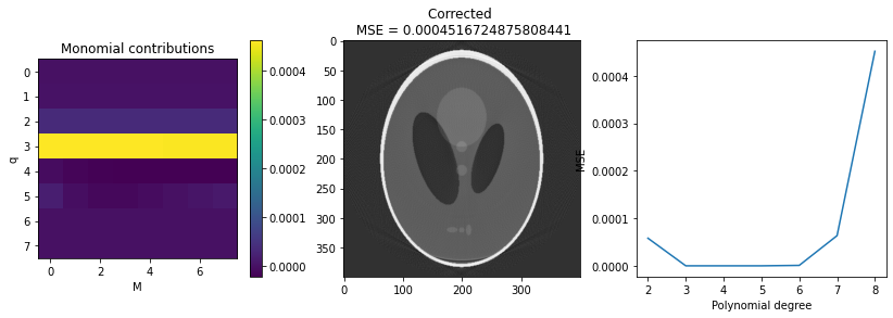
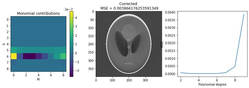
Let’s visualize the coefficients to see what basis images contribute the most
Recall the correction is \(\hat{p} = c_{i,j} q^i M^j\) thus the coordinates in the image below indicate the monomial and its relative contribution to the polynomial
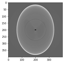
def correctAndDisplay(corrupted_r, m, c, theta): p = performCorrection2D(corrupted_r, m, c) corrected = iradon(p, theta=theta, circle=True) plt.imshow(corrected, cmap=plt.cm.Greys_r) ms_error = mse(corrected,ideal) plt.title("Corrected \n MSE = "+str(ms_error))return ms_errorcorrectAndDisplay(corrupted_r, m, c, theta)
Finally repeat once more with Beam hardening strength set to zero and spatiall varying strength on max, how does this affect the coefficient activation map?
Observe how the MSE decreases then increases at higher degrees. This demonstrates a weakness of Vandermonde polynomial interpolation that as the Vandermonde matrix becomes larger its condition number grows dramatically and the result becomes unstable.
Move on to the last notebook on iterative methods for solving the Vandermonde interpolation least squares problem: https://colab.research.google.com/drive/1kErNKAbJlJUpq2jsb0roMJA7kTNB9vY0